Introduction
A data set was obtained from the UC Irvine Machine Learning Repository and contains information regarding kernels from three different varieties of wheat (Kama, Rosa, and Canadian). A total of 210 kernels were included, with each wheat class being represented by 70 specimens. In addition to the type of wheat, there are seven variables included in this data set: (1) area, (2) perimeter, (3) compactness, (4) length, (5) width, (6) asymmetry coefficient, and (7) length of kernel groove. The objective of this project was to determine how these three varieties could be distinguished by conducting several multivariate analyses in R. A correlation matrix, principal component analysis (PCA), and a linear discriminant analysis (LDA) were explored.
Correlation Matrix
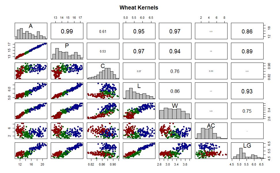
Figure 1 A correlation matrix plot of the data set. The wheat varieties are represented by color. Blue is Rosa; green is Kama; red is Canadian. The variables are indicated within the histograms. A is area; P is perimeter; C is compactness; L is length; W is width; AC is asymmetry coefficient; LG is length of kernel groove.
The three varieties appear to cluster together in every scatterplot in figure 1, indicating that all the variables included in the data set will be useful in distinguishing the types of wheat. This decision was tested by performing multiple linear discriminant analyses, each using different combinations of the seven variables. As expected, the most accurate model included all variables. There are strong linear relationships among most of the variables, with correlation coefficients ranging from 0.75 to 0.99. However, there is much more scatter in the compactness (C) and the asymmetry coefficient (AC) variables, and the relationships are nonlinear. As a result, the correlation coefficients are typically much smaller. It is likely that these two variables are not well correlated with the rest of the data because they are the only variables that are not measurements of kernel size. The three wheat varieties still cluster together in the scatterplots of these variables so they will be retained for further analyses.
The three varieties appear to cluster together in every scatterplot in figure 1, indicating that all the variables included in the data set will be useful in distinguishing the types of wheat. This decision was tested by performing multiple linear discriminant analyses, each using different combinations of the seven variables. As expected, the most accurate model included all variables. There are strong linear relationships among most of the variables, with correlation coefficients ranging from 0.75 to 0.99. However, there is much more scatter in the compactness (C) and the asymmetry coefficient (AC) variables, and the relationships are nonlinear. As a result, the correlation coefficients are typically much smaller. It is likely that these two variables are not well correlated with the rest of the data because they are the only variables that are not measurements of kernel size. The three wheat varieties still cluster together in the scatterplots of these variables so they will be retained for further analyses.
Principal Component Analysis
A principal component analysis (PCA) was performed to find the principal components that represent most of the variation in the data and reduce the dimensionality of the data set. First, the data was standardized so that it has a variance of 1 and a mean of 0 to prevent the variables with the most variance from biasing the PCA. To decide how many principal components should be retained, a scree plot of the components was created (figure 2). Under Kaiser’s criterion, the principal components of standardized data that have a variance greater than 1 should be retained (Coghlan 2010). Therefore, the loadings for only principal components 1 and 2 were analyzed, which explained 89% of the variance. Variables A, P, L, W, and LG load together on the first principal component because they have very similar values (approximately -0.4). Thus, the first principal component indicates the size of the wheat kernels. The second principal component represents a negative correlation between C and AC because their loadings have high absolute values but opposite signs (-0.529 and 0.717 respectively). It is not surprising that variables C and AC did not load on the same principal component as the other variables because they are the only variables in the data set that are not indicators of kernels size.
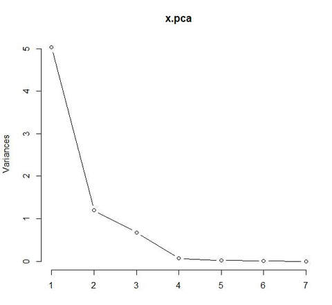
Figure 2 A scree plot showing the variance (y-axis) for each principal component (x-axis).
|
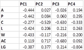
Table 1 Loadings for each variable for the first four principal components.
|
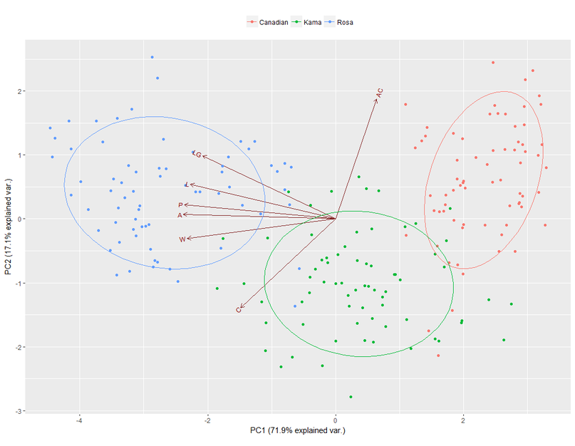
Figure 3 A plot of the first and second principal components showing the vector of each variable and the three wheat varieties.
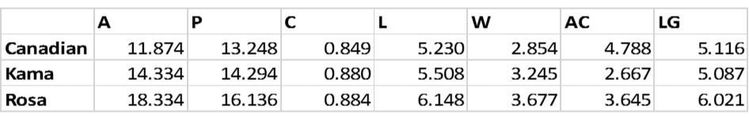
Table 2 Mean values among wheat varieties
The first principal component was able to separate the Canadian and Rosa varieties well. Figure 3 suggests that the Rosa variety will be the largest type of kernel, and the Canadian variety will be the smallest while the Kama group typically falls in the middle. This interpretation is confirmed upon examination of the mean group values for the variables (table 2). The second principal components did not separate the Canadian and Rosa varieties, but the Kama variety was distinguished by generally lower PCA values. Figure 3 suggests that the Kama variety will have lower AC values than the other two groups, meaning that it will be more spherical. Once again, this is confirmed by the mean values in table 2.
The first principal component was able to separate the Canadian and Rosa varieties well. Figure 3 suggests that the Rosa variety will be the largest type of kernel, and the Canadian variety will be the smallest while the Kama group typically falls in the middle. This interpretation is confirmed upon examination of the mean group values for the variables (table 2). The second principal components did not separate the Canadian and Rosa varieties, but the Kama variety was distinguished by generally lower PCA values. Figure 3 suggests that the Kama variety will have lower AC values than the other two groups, meaning that it will be more spherical. Once again, this is confirmed by the mean values in table 2.
Linear Discriminant Analysis
A linear discriminant analysis (LDA) was performed on this data set to find discriminant functions that can separate the kernels into their respective wheat varieties using the seven variables. The maximum number of discriminant functions that can be used is one less than the number of wheat varieties (Coghlan 2010). Thus, two discriminant functions were produced in this analysis. The data set was first randomized and then split in half. The first half was used as a training set while the second half was used to test the accuracy of the LDA. This was done to ensure that the misclassification rate of the LDA was accurate. If the LDA was tested with the same data that was used to train it, the misclassification rate would be erroneously low. Unlike the PCA, the data set was not standardized before performing the LDA because the values of the linear discriminant functions are the same regardless of whether the data is standardized (Coghlan 2010).
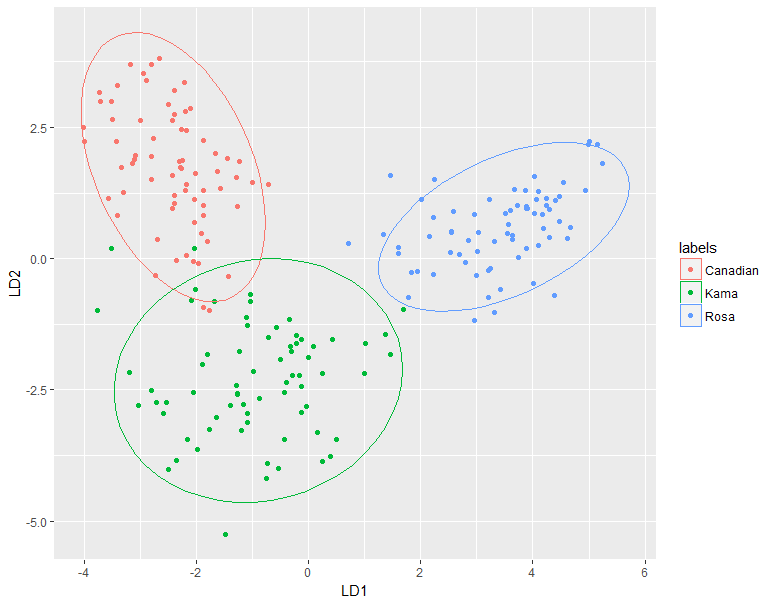
Figure 4 A plot of the values for the first and second discriminant functions.
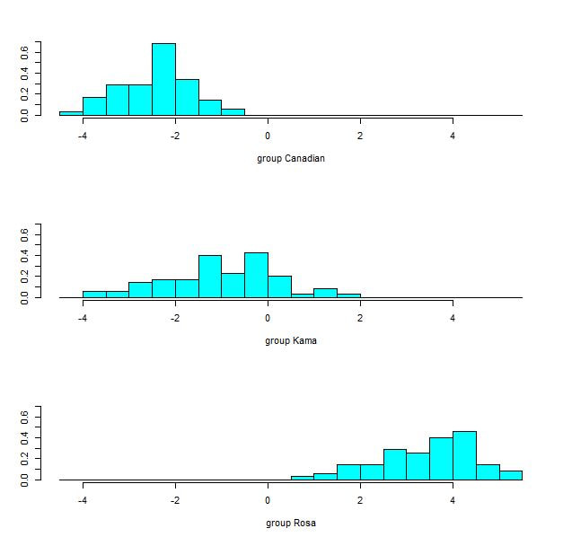
Figure 5. Histograms of the first discriminant function values for each wheat variety.
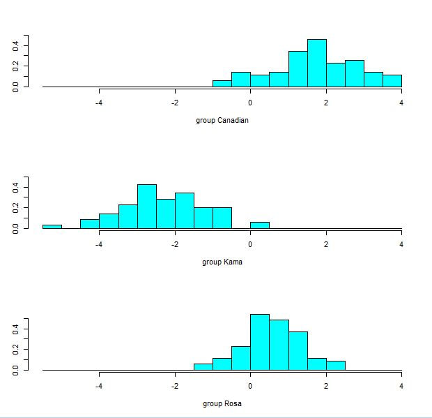
Figure 6 Histograms of the second discriminant function values for each wheat variety.
The percentage of separation achieved by the first and second discriminant function was 70.5% and 29.5% respectively. The first linear discriminant function was able to separate the Canadian and Rosa varieties completely (figures 4 and 5). However, the Kama variety was not easily distinguished. The histogram for the Kama group greatly overlap with the histograms of the Canadian group on the left and the Rose group on the right. However, the second linear discriminant function was able to distinguish the Kama variety more successfully (figure 6). Therefore, both functions should be used to distinguish wheat varieties. The LDA misclassified 4 kernels, which resulted in an error rate of 3.8%. Three Kama kernels were misclassified as Canadian, and one Rosa kernel was misclassified as Kama. It is not surprising that zero Rosa kernels were misclassified as Canadian and vice versa because of the degree of separation achieved between these groups.
A more general method for distinguishing the wheat varieties is to create allocation rules based upon the midpoints between the mean values of the linear discriminant function for each group. Since the first function was able to separate Rosa and Canadian varieties, the midpoints of the first function should be used to create allocation rules for these two groups. Because the second function achieved better separation for the Kama group, it should be used to classify the Kama variety. The misclassification rate for these allocation rules (listed below) was 9.5%. Three Canadian kernels were misclassified as Kama; two Kama kernels were misclassified as Rosa, and five Rosa kernels were misclassified as Kama. Once again, every error involves the Kama group because Rosa and Canadian varieties were completely separated by the LDA.
A more general method for distinguishing the wheat varieties is to create allocation rules based upon the midpoints between the mean values of the linear discriminant function for each group. Since the first function was able to separate Rosa and Canadian varieties, the midpoints of the first function should be used to create allocation rules for these two groups. Because the second function achieved better separation for the Kama group, it should be used to classify the Kama variety. The misclassification rate for these allocation rules (listed below) was 9.5%. Three Canadian kernels were misclassified as Kama; two Kama kernels were misclassified as Rosa, and five Rosa kernels were misclassified as Kama. Once again, every error involves the Kama group because Rosa and Canadian varieties were completely separated by the LDA.
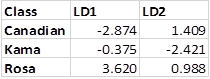
Table 3 Mean values of the linear discriminant functions.
|
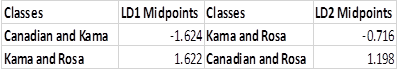
Table 4 Midpoints of the linear discriminant functions between groups.
|
Allocation Rules
- If the first discriminant function is ≤ -1.624, predict the kernel to be Canadian.
- If the second discriminant function is > -0.7164 and ≤ 1.198, predict the kernel to be Kama.
- If the first discriminant function is > 1.622, predict the kernel to be Rosa.
Conclusions
The correlation matrix plot (figure 1), the PCA, and the LDA all indicate that varieties of wheat kernels can be distinguished by their size, their asymmetry coefficients (AC) and their compactness (C). Rosa is the largest type of wheat kernel, and the Canadian variety is the smallest while Kama is intermediate, making it difficult to distinguish. However, the Kama variety has the smallest AC values, meaning that its shape is more spherical than the other groups. This is supported by the fact that the Kama group has the smallest difference between the average length (L) and width (W) values (table 2) among the three varieties. The Canadian group can also be distinguished by its low average C value whereas Rosa and Kama kernels have higher and very similar C values. These distinctions made it possible for the LDA separate the three groups (figure 4). However, variance among the groups makes it impossible to confidently predict the wheat variety of every kernel in the test data set. As a result, the LDA had a misclassification rate of 3.8%. These errors all involved the Kama variety because its ranges for all of the variables included in the data set overlapped with the ranges of the Canadian and Rosa varieties. However, there was no overlap between the Canadian and Rosa kernels, resulting in no misclassifications of Canadian kernels for Rosa kernels or vice versa. This held true for the allocation rules as well. However, the misclassification rate was 9.5% because the allocation rules are simple generalizations derived from the mean values of the linear discriminant functions.
